Chapter 3 Using dplR
This document describes basic features of dplR by following the initial steps that an analyst might follow when working with a new tree-ring data set. The document starts with reading in ring widths and plotting them. We describe a few of the available methods for detrending and then show how to extract basic descriptive statistics. We show how to build and plot a simple mean-value chronology. We also show how to build a chronology using the expressed population signal from the detrended ring widths as an example of how more complicated analysis can be done using dplR.
3.1 What is Covered
The Dendrochronology Program Library in R (dplR) is a package for dendrochronologists to handle data processing and analysis. This document gives just a brief introduction of some of the most commonly used functions in dplR. There is more detailed information available in the help files and in the literature (Bunn, 2008).
In this document, we will walk through the most basic activities of working with tree-ring data in roughly the order that a user might follow. E.g., reading data, detrending, chronology building, and doing preliminary exploratory data analysis via descriptive statistics.
3.2 Working with Ring-Width Data
3.2.1 Reading Data
There are many ways that tree-ring data are digitally stored. These range in sophistication from the simple (and commonly used) Tucson/decadal format file of ring widths to the more complex (but richer) TRiDaS format. The type of data used most often by dendrochronologists is a series of ring widths from tree cores. We generally refer to these as rwl objects for “ring width length” but there is no reason these cannot be other types of tree-ring data (e.g., density).
The workhorse function for getting tree-ring data into R is dplR’s read.rwl function. This function reads files in "tucson", "compact", "tridas", and "heidelberg" formats. The on-board rwl data sets in dplR (i.e., co021, ca533, gp.rwl) were all imported into R using this function.
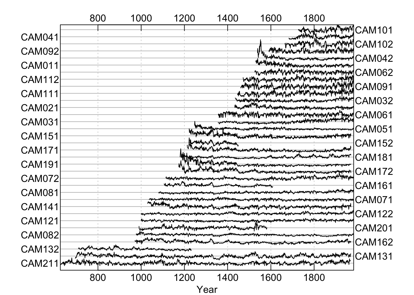
Throughout this document we will use the on-board data set ca533 which gives the raw ring widths for bristlecone pine Pinus longaeva at Campito Mountain in California, USA. There are 34 series spanning 1358 years.
These objects are structured very simply as a data.frame with the series in columns and the years as rows. The series IDs are the column names and the years are the row names (both stored as characters). For instance, using the Campito Mountain ring widths we can load the data and learn some basic things about it:
## [1] 1358## [1] 34We can look a little deeper at this object (ca533) and get the series names as well as look at the time values associates with the data:
##  [1] "CAM011" "CAM021" "CAM031" "CAM032" "CAM041" "CAM042" "CAM051" "CAM061"
##  [9] "CAM062" "CAM071" "CAM072" "CAM081" "CAM082" "CAM091" "CAM092" "CAM101"
## [17] "CAM102" "CAM111" "CAM112" "CAM121" "CAM122" "CAM131" "CAM132" "CAM141"
## [25] "CAM151" "CAM152" "CAM161" "CAM162" "CAM171" "CAM172" "CAM181" "CAM191"
## [33] "CAM201" "CAM211"## [1] 626 627 628 629 630 631 632 633 634 6353.2.2 Describing and Plotting Ring-Width Data
Once a rwl data set has been read into R, there are a variety of ways to describe and visualize those data. Take note that this object is stored both as a generic data.frame in R but it also is part of a special class called rwl which will let R know how to do some special things with it like summarize and plot the data:
## [1] "rwl" "data.frame"Thus, we can plot a rwl object by showing either the segments arranged over time as straight lines or as a “spaghetti plot”. The rwl objects have generic S3 methods for plot and summary meaning that R knows how to do something special when plot or summary are invoked on an object with class rwl. E.g.,:
3.3 Descriptive Statistics
The simplest report on a rwl object can be print to the screen via:
## Number of dated series: 34
## Number of measurements: 23276
## Avg series length: 684.5882
## Range:  1358
## Span:  626 - 1983
## Mean (Std dev) series intercorrelation: 0.6294255 (0.0859289)
## Mean (Std dev) AR1: 0.7092647 (0.09811876)
## -------------
## Years with absent rings listed by series
##     Series CAM011 -- 1753 1782
##     Series CAM031 -- 1497 1500 1523 1533 1540 1542 1545 1578 1579 1580 1655 1668 1670 1681
##     Series CAM032 -- 1497 1523 1579 1654 1670 1681 1782
##     Series CAM051 -- 1475
##     Series CAM061 -- 1497 1523 1542 1545 1547 1579 1654 1655 1668 1670 1672 1782 1858 1960
##     Series CAM062 -- 1542 1545 1547 1548 1579 1654 1655 1670 1672 1782 1836 1857 1858 1929
##     Series CAM071 -- 1269 1497 1498 1523 1542 1547 1578 1579 1612 1655 1656 1668 1670 1672 1674 1690 1707 1708 1756 1782 1795 1820 1836 1845 1857 1858 1924 1948 1960
##     Series CAM072 -- 1218 1497 1498 1523 1533 1538 1542 1545 1546 1547 1571 1579 1580 1590 1654 1655 1668 1670 1672 1675 1690
##     Series CAM081 -- 1218 1336
##     Series CAM082 -- 1362 1858 1865
##     Series CAM091 -- 1655 1669 1670 1782 1858
##     Series CAM092 -- 1624 1654 1655 1670 1672 1675 1677 1690 1703 1705 1707 1708 1710 1733 1753 1756 1757 1774 1777 1781 1782 1783 1784 1795 1807 1824 1829 1836 1845 1857 1858 1899 1904 1929 1936 1961
##     Series CAM101 -- 1782 1783 1899 1929
##     Series CAM102 -- 1669 1690 1782 1858 1899 1929
##     Series CAM111 -- 1542
##     Series CAM112 -- 1542
##     Series CAM121 -- 1093 1218 1254 1361 1365 1460 1462 1468 1473 1475 1492 1497 1542 1544 1545 1547 1600 1899 1960
##     Series CAM122 -- 1117 1133 1147 1177 1218 1254 1361 1475 1497 1670
##     Series CAM131 -- 1361
##     Series CAM151 -- 1670 1703
##     Series CAM161 -- 1523
##     Series CAM162 -- 1618 1624 1641
##     Series CAM181 -- 1450 1523
##     Series CAM191 -- 1475 1497 1523 1533 1542 1558 1571 1578 1618 1655 1668 1670 1675 1677 1690 1705 1777 1929
##     Series CAM201 -- 1523
##     Series CAM211 -- 645 762 809 847 924 957 1014 1118 1123 1133 1147 1189 1350 1384 1468 1571 1641
## 234 absent rings (1.005%)
## -------------
## Years with internal NA values listed by series
##     None
That’s pretty basic information. We can look at some common (and not-so common) descriptive statistics of a rwl object:
ca533.stats <- summary(ca533) # same as calling rwl.stats(ca533)
head(ca533.stats,n=5) # look at the first five series
## series first last year mean median stdev skew gini ar1
## 1 CAM011 1530 1983 454 0.440 0.40 0.222 1.029 0.273 0.696
## 2 CAM021 1433 1983 551 0.424 0.40 0.185 0.946 0.237 0.701
## 3 CAM031 1356 1983 628 0.349 0.29 0.214 0.690 0.341 0.808
## 4 CAM032 1435 1983 549 0.293 0.26 0.163 0.717 0.309 0.661
## 5 CAM041 1683 1983 301 0.526 0.53 0.223 0.488 0.238 0.690These are common summary statistics like mean, median, etc. but also statistics that are more specific to dendrochronology like the first-order autocorrelation (ar1), gini (gini). Note that output object ca533.stats is itself a data.frame and its data can be used to plot, summarize, etc.
For instance, we can get the mean and standard deviation of segment length via:
## [1] 684.5882## [1] 276.9972Or, we can look at the spread of the first-order autocorrelation via summary(ca533.stats$ar1) or make a plot to show the data. Here we will demonstrate a somewhat involved plot to get you an idea of how to layer plotting commands:
boxplot(ca533.stats$ar1,ylab=expression(phi[1]),col = "lightblue")
stripchart(ca533.stats$ar1, vertical = TRUE,
    method = "jitter", jitter = 0.02,add = TRUE, pch = 20, col = 'darkblue',cex=1.25)
ar1Quant <- quantile(ca533.stats$ar1,probs = c(0.25,0.5,0.75))
abline(h=ar1Quant,lty="dashed",col="grey")
mtext(text = names(ar1Quant),side = 4,at = ar1Quant,las=2)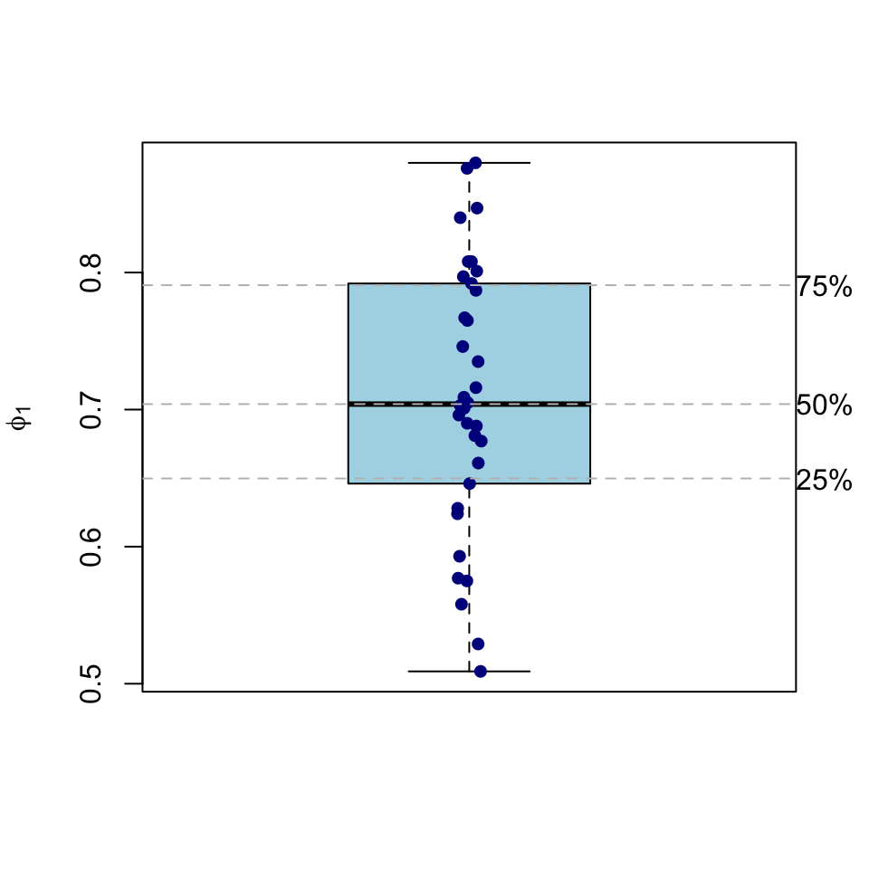
Quick editorial note. I’ve switched from base R plotting to using ggplot in most all of my work. I need to go through and provide new plotting examples for everything, but time is short. Real quick though, here is a ggplot
library(ggplot2)
ar1 <- data.frame(x="CA 533",y=ca533.stats$ar1)
ggplot(ar1,aes(x,y)) + geom_boxplot(width=.2) +
  geom_jitter(width=0.1) +
  labs(y=expression(phi[1]),x=element_blank()) +
  theme_minimal()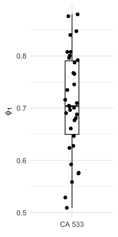
There are a few other descriptive stats that are available. Mean sensitivity (sens1 and sens2) used to be included in the standard summary statistics but mean sensitivity is actually a terrible statistic that should rarely, if ever, be used (Bunn et al., 2013). It is at best equivalent to the standard deviation of a time series in cases without high autocorrelation and is an inefficient estimator of the coefficient of variation. So use cautiously if at all.
3.4 Detrending
Analysts often (but not always) detrend a rwl data set to create an object containing ring-width index (rwi) values. The dplR package contains most standard detrending methods including detrending via splines, fitting negative exponential curves, and so on. There are also dplR functions for less commonly used detrending methods like regional curve and signal-free standardization.
A rwi object has the same basic properties as the rwl object from which it is made. I.e., it has the same number of rows and columns, the same names, and so on. The difference is that each series has been standardized by dividing the ring widths against a growth model (e.g., a stiff spline, a negative exponential, etc.). This gives each series a mean of one (thus referred to as “indexed”) and allows a chronology to be built (next section). As read.rwl is the primary function for getting data into R, detrend is the primary function for standardizing rwl objects (but see cms, rcs, bai.in, and bai.out as well).
3.4.1 Common Detrending Methods
As any dendrochronologist will tell you, detrending is a dark art. In dplR we have implemented some of the standard tools for detrending but all have drawbacks. In all of the methods, the detrending is the estimation and removal of the low frequency variability that is due to biological or stand effects. The standardization is done by dividing each series by the growth trend to produce units in the dimensionless ring-width index (RWI). Much of the text that follows is modified from the help page of detrend.
Probably the most common method for detrending is what is often called the “conservative” approach of attempting to fit a negative exponential curve to a series. In the dplR implementation the "ModNegExp" method of detrend attempts to fit a classic nonlinear model of biological growth of the form \((f(t) = a \times \mathrm{e}^{bt} + k)\), where the argument of the function is time, using nls. See Fritts (2001) for details about the parameters. If a suitable nonlinear model cannot be fit (function is non-decreasing or some values are not positive) then a linear model is fit using lm. That linear model can have a positive slope unless pos.slope is FALSE in which case the series is standardized by its mean (method "Mean" in detrend).
For instance, every series in the ca533 object can be detrended at once with an age-dependent spline via:
This saves the results in ca533.rwi which is a data.frame with the same dimensions as the rwl object ca533 and each series standardized.
## [1] 1358## [1] 34## CAM011 CAM021 CAM031 CAM032 CAM041 CAM042 CAM051 CAM061
## 1.0631050 1.0224109 2.2693152 1.3842987 1.0406039 1.0705729 0.9986579 1.0271454
## CAM062 CAM071 CAM072 CAM081 CAM082 CAM091 CAM092 CAM101
## 0.9972379 1.0019581 1.3751516 1.3000696 0.9988440 1.1558844 1.1102479 1.4626404
## CAM102 CAM111 CAM112 CAM121 CAM122 CAM131 CAM132 CAM141
## 1.0631347 1.1279841 1.0140838 1.3058103 1.0625794 1.1127666 0.9997782 1.0105626
## CAM151 CAM152 CAM161 CAM162 CAM171 CAM172 CAM181 CAM191
## 1.1363804 0.9990169 0.9992451 1.1053696 1.0649315 1.0242845 1.5740168 1.0651213
## CAM201 CAM211
## 1.0478775 1.1227146When detrend is run on a rwl object the function loops through
each series. It does this by calling a different function
(detrend.series) for each column in the rwl object.
But, a user can also call detrend.series and it is useful to do so here
for educational purposes.
Let us detrend a single series and apply more than one detrending method when we call the detrend function. We will call detrend.series using the verbose mode so that we can see the parameters applied for each method. The detrend.series function produces a plot by default.
##  ~~~~~~~~~~~~~~~~~~~~~~~~~~~~~~~~~~~~~~~~~~~~~~~~~~~~~~~~~~~~~~~~~~~~~~~~~~~~~~
## Verbose output:
##
##  ~~~~~~~~~~~~~~~~~~~~~~~~~~~~~~~~~~~~~~~~~~~~~~~~~~~~~~~~~~~~~~~~~~~~~~~~~~~~~~
##  Options
##  make.plot      TRUE
##  method(s)1     c("Spline", "ModNegExp", "Mean", "Ar", "Friedman", "ModHugershoff",
##  method(s)2     "AgeDepSpline")
##  nyrs           NULL
##  f              0.5
##  pos.slope      FALSE
##  constrain.nls  never
##  verbose        TRUE
##  return.info    FALSE
##  wt             default
##  span           cv
##  bass           0
##  difference     FALSE
##
##  ~~~~~~~~~~~~~~~~~~~~~~~~~~~~~~~~~~~~~~~~~~~~~~~~~~~~~~~~~~~~~~~~~~~~~~~~~~~~~~
##  Zero indices in input series:
##  1128 1157
##
##  ~~~~~~~~~~~~~~~~~~~~~~~~~~~~~~~~~~~~~~~~~~~~~~~~~~~~~~~~~~~~~~~~~~~~~~~~~~~~~~
##  Detrend by ModNegExp.
##  Trying to fit nls model...
##  nls coefs
##  a:  0.66109686
##  b: -0.01184415
##  k:  0.31793386
##
##  ~~~~~~~~~~~~~~~~~~~~~~~~~~~~~~~~~~~~~~~~~~~~~~~~~~~~~~~~~~~~~~~~~~~~~~~~~~~~~~
##  Detrend by ModHugershoff.
##  Trying to fit nls model...
##  nls coefs
##  a: 0.45550002
##  b: 0.15419657
##  g: 0.01532032
##  d: 0.32391578
##
##  ~~~~~~~~~~~~~~~~~~~~~~~~~~~~~~~~~~~~~~~~~~~~~~~~~~~~~~~~~~~~~~~~~~~~~~~~~~~~~~
##  Detrend by age-dependent spline.
##  Spline parameters
##  nyrs = 50, pos.slope = FALSE
##
##  ~~~~~~~~~~~~~~~~~~~~~~~~~~~~~~~~~~~~~~~~~~~~~~~~~~~~~~~~~~~~~~~~~~~~~~~~~~~~~~
##  Detrend by spline.
##  Spline parameters
##  nyrs = 304, f = 0.5
##
##  ~~~~~~~~~~~~~~~~~~~~~~~~~~~~~~~~~~~~~~~~~~~~~~~~~~~~~~~~~~~~~~~~~~~~~~~~~~~~~~
##  Detrend by mean.
##  Mean =  0.4395859
##
##  ~~~~~~~~~~~~~~~~~~~~~~~~~~~~~~~~~~~~~~~~~~~~~~~~~~~~~~~~~~~~~~~~~~~~~~~~~~~~~~
##  Detrend by prewhitening.
## Call:
## ar(x = y[idx.goody])
##
## Coefficients:
##       1        2        3        4        5        6        7        8
##  0.3884   0.1393   0.0002   0.0838   0.1321   0.0613   0.0381  -0.1255
##       9       10       11       12       13       14       15       16
##  0.0366  -0.0996  -0.0102   0.0147   0.0879   0.0104   0.0639  -0.0132
##      17       18       19       20       21       22       23
##  0.0151  -0.0044  -0.0539   0.1240  -0.0302  -0.0545   0.1370
##
## Order selected 23  sigma^2 estimated as  0.02092
##  ~~~~~~~~~~~~~~~~~~~~~~~~~~~~~~~~~~~~~~~~~~~~~~~~~~~~~~~~~~~~~~~~~~~~~~~~~~~~~~
##  Fits from method=='Ar' are not all positive.
##   Setting values <0 to 0 before rescaling.
##   This might not be what you want.
##   ARSTAN would tell you to plot that dirty dog at this point.
##   Proceed with caution.
##  ~~~~~~~~~~~~~~~~~~~~~~~~~~~~~~~~~~~~~~~~~~~~~~~~~~~~~~~~~~~~~~~~~~~~~~~~~~~~~~
##
##  ~~~~~~~~~~~~~~~~~~~~~~~~~~~~~~~~~~~~~~~~~~~~~~~~~~~~~~~~~~~~~~~~~~~~~~~~~~~~~~
##  Detrend by Friedman's super smoother.
##  Smoother parameters
##  span = cv, bass = 0
##  wt = default
##
##  ~~~~~~~~~~~~~~~~~~~~~~~~~~~~~~~~~~~~~~~~~~~~~~~~~~~~~~~~~~~~~~~~~~~~~~~~~~~~~~
##  Zero indices in Ar series:
##  993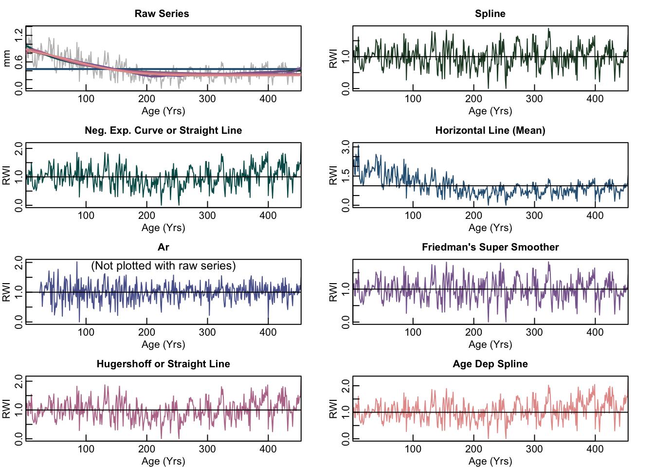
Note that advanced users can use return.info=TRUE to have all the fitting parameters returned in a list. Having access to these is occasionally desirable.
3.4.2 Interactive detrending
There are many instances where a user needs fine scale control while detrending perhaps fitting a negative exponential curve to one series, a spline to another, and the mean to a third. Like with crossdating, interactive detrending is a case where an app is useful. The iDetrend app is relatively simple interface to detrend.series that let’s users fit curves and plot them with several different options. When completed the user can save a file with the detrended data as well as generate log file that allows reproduction of the detrending from the command line. It’s available here
3.4.3 Other Detrending Methods
There are other detrending methods that are less commonly used but might have theoretical advantages. These include regional curve standardization (function rcs), C-Method Standardization (function cms), and converting measurements of ring widths to basal area increment (functions bai.in and bai.out). See their help pages for further information.
3.5 Descriptive Statistics for Detrended Data
It is also easy in dplR to compute commonly used descriptive statistics that describe the correlation between series (both within and between tree correlations) as well as the expressed population signal, signal-to-noise ratio, and subsample signal strength for a data set. These are done in dplR using the rwi.stats function so-named because these statistics are typically (but not always) carried out on detrended and standardized ring widths (rwi). If a data set has more than one core taken per tree this information can be used in the calculations to calculate within vs. between tree correlation. The function read.ids is used to identify which trees have multiple cores.
##   n.cores n.trees  n n.tot n.wt n.bt rbar.tot rbar.wt rbar.bt c.eff rbar.eff
## 1      34      21 21   523   13  510    0.445   0.606    0.44 1.448    0.502
##     eps    snr
## 1 0.955 21.128
There is (at least) one other way of looking at the average interseries correlation of a data set. The interseries.cor function in dplR gives a measure of average interseries correlation that is different from the rbar statistics from rwi.stats. In this function, correlations are calculated serially between each tree-ring series and a master chronology built from all the other series in the rwl object (leave-one-out principle). The average of those correlations is sometimes called the “overall interseries correlation” or even the “COFECHA correlation” in reference to commonly used crossdating software COFECHA. This number is typically higher than the various rbar values given by rwi.stats. We are showing just the first five series and the mean for all series here:
##          res.cor p.val
## CAM011 0.5324769     0
## CAM021 0.6826813     0
## CAM031 0.5148129     0
## CAM032 0.6311426     0
## CAM041 0.5007524 0## [1] 0.6381676Again, if these concepts are unknown to you statistically look at some of the canonical works in dendrochronology like Cook et al. (1990), Fritts (2001), and Hughes et al. (2011).
3.6 Building a Mean-Value Chronology
After detrending, a user will typically build a chronology by averaging across the years of the rwi object. In dplR the function for doing this is chron which by default uses Tukey’s biweight robust mean (an average that is unaffected by outliers).
This object has the same number of rows as the rwi object that was used as the input and two columns. The first gives the chronology and the second the sample depth (the number of series available in that year).
## [1] 1358 34## [1] 1358 2An object produced by chron has a generic S3 method for plotting which calls the crn.plot function (which has many arguments for customization). Here we will just make a simple plot of the chronology with a smoothing spline (function caps) added.
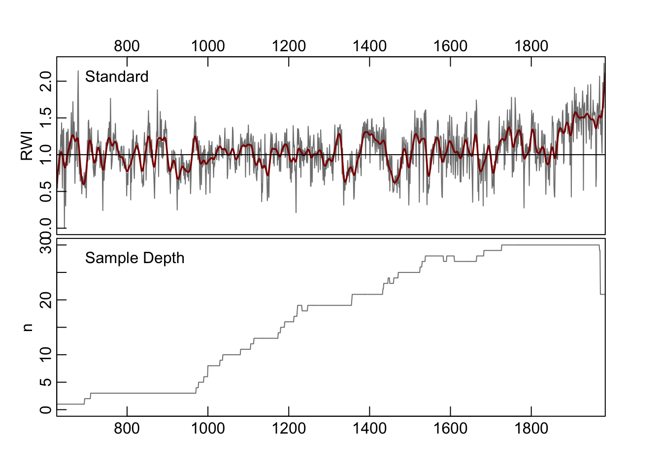
The chron function is the most basic (and most common) way to buld a chronology but there are many other ways as we will see in the next few chapters.
3.7 Conclusion
In general this page aims to give a very cursory overview of basic tasks that most dendrochronologists will want to be aware of. Know that we are just scratching the surface of what dplR is capable of. Browsing the list of functions in dplR will give you an idea of what else is available.