dplpy User Manual
Welcome to the dplpy user manual
Here is a list of functions (in alphabetical order) with descriptions:
| Function | Description |
|---|---|
ar_func |
Fits series to autoregressive (AR) models and related functions |
autoreg |
Fits series to autoregressive (AR) models and related functions |
chron |
Creates a mean value chronology for a dataset, typically the ring width indices of a detrended series |
detrend |
Detrends a given series or data frame, first by fitting data to curve(s), with spline(s) as the default, and then by calculating residuals or differences compared to the original data. |
help |
Displays help (alpha). |
plot |
Generates line, spaghetti or segment plots. |
rbar |
Finds best interval of overlapping series over a period of years, and calculating rbar constant for a dataset over period of overlap. |
readers |
Reads data from supported file types (*.CSV and *.RWL) and stores them in dataframe. |
readme |
Goes to this website. |
report |
Generates a report about absent rings in the data set. |
series_corr |
Crossdating function that focuses on the comparison of one series to the master chronology. |
stats |
Generates summary statistics for RWL and CSV format files. |
summary |
Generates a summary for RWL and CSV format files. |
xdate |
Crossdating function for dplPy loaded datasets. |
ar_func
Summary
Main function for autoregressive (AR) modeling.
Returns residuals and mean of best AR fit with specified lag.
Parameters
-
data:str- a data file (.CSVor.RWL) or a pandas dataframe imported fromdpl.readers(). -
series:str- an individual series within a chronologydatafile. -
lag:intdefault5- nuber of years.
Examples
>>> dpl.ar_func(<data>["<series>"], <lag number>)
>>> dpl.ar_func(ca533["CAM191"], 10)
In the above example, we use dataset look at dataset ca533 series CAM191 and specified a lag of 10.
Returns
Users can expect an array of residuals + mean for selected series.
The expected output from the example above will look similar to this:
array([ 0.71130658, -0.23204695,  0.52121028,  0.57597523,  0.90108448,
        0.20495808, -0.23457629,  0.58819405,  0.66478718,  0.47521983,
        0.92695177, -0.35659493,  0.42220031, -0.19197698, -0.08828572,
        0.5320343 ,  0.28471761,  0.39486259,  0.10748019,  0.25214937,
        0.46500727,  1.45016901,  0.28605889,  0.29470389,  0.34120629,
    -0.31249819,  0.42380461,  0.23473108, -0.06796468,  0.38897624,
        0.68666198,  0.77677716,  0.62360082,  0.43398575,  0.74032758,
        0.5880663 ,  0.20567916,  0.23525549,  0.63297387,  0.94101874,
        0.06615244,  0.73838454,  0.51092414,  0.25087689,  0.3873105 ,
        0.48383716,  0.28317419,  0.46750972,  0.60187677,  0.40542752,
        0.54822178,  0.08560112,  0.26122762,  0.13318504,  0.25876284,
        0.56315817,  0.40823334,  0.36114307,  0.49613157,  0.4169329 ,
        0.40733772,  0.25578201,  0.42718681,  0.59555259, -0.21075308,
        0.11587297,  0.62082607,  0.65467697, -0.17674732,  0.56107325,
        0.51825623,  0.58111792,  0.61318262,  0.3742455 ,  0.07211766,
        0.01136486,  0.06596661,  0.32254786,  0.39898574,  0.22616678,
        0.34727753,  0.42409955,  0.51594014,  0.23294973,  0.50911683,
        0.84802911,  0.48218982,  0.393356  ,  0.22153173,  0.65209051,
        0.48231136,  0.19053267,  0.39660363,  0.39800466,  0.29138228,
    -0.030384  ,  0.49157549,  0.49579055,  0.25640508,  0.48196172,
        0.28278419,  0.53502938,  0.41559126,  0.34577752,  0.33023954,
        0.55383387,  0.4391052 ,  0.35063736,  0.20157626,  0.25298519,
        0.51312838,  0.53184596,  0.43997298,  0.27903576,  0.43143646,
        0.45186539,  0.3734363 ,  0.41050279,  0.67168476,  0.31693981,
        0.32281309,  0.5155617 ,  0.51985799,  0.48651392,  0.50650445,
...
        0.39541278,  0.47066705,  0.34558178,  0.46008747,  0.34158785,
        0.3672973 ,  0.37749446,  0.34939726,  0.37388067,  0.4241256 ,
        0.23815543,  0.29207569,  0.47247813,  0.44170539,  0.4410876 ,
        0.4007522 ,  0.29655365,  0.38460918,  0.39774193,  0.42761775,
        0.38384653])
autoreg
Summary
Secondary function for AR modeling. Returns parameters of best fit AR model with specified lag.
Best AR model is selected based on AIC value.
Parameters
-
data:str- a data file (.CSVor.RWL) or a pandas dataframe imported fromdpl.readers(). -
series:str- an individual series within a chronologydatafile. -
lag:intdefault5- nuber of years.
Note
This function and its outputs are integrated in the ar_func function.
Examples
>>> import dplpy as dpl
>>> data = dpl.readers("../tests/data/csv/ca533.csv")
>>> dpl.autoreg(data['series name']) -> returns parameters of best fit AR model
                                        with maxlag of 5 (default) or other
                                        specified number
dpl.autoreg(ca533["CAM191"], 10)
Returns
A table listing autoregressive paramenters for the specified series;
The expected output from the example above will look similar to this:
const         0.022210
CAM191.L1     0.503373
CAM191.L2     0.087230
CAM191.L3     0.143716
CAM191.L4     0.020119
CAM191.L5    -0.027769
CAM191.L6    -0.010029
CAM191.L7     0.001373
CAM191.L8     0.025588
CAM191.L9     0.042340
CAM191.L10    0.136916
dtype: float64
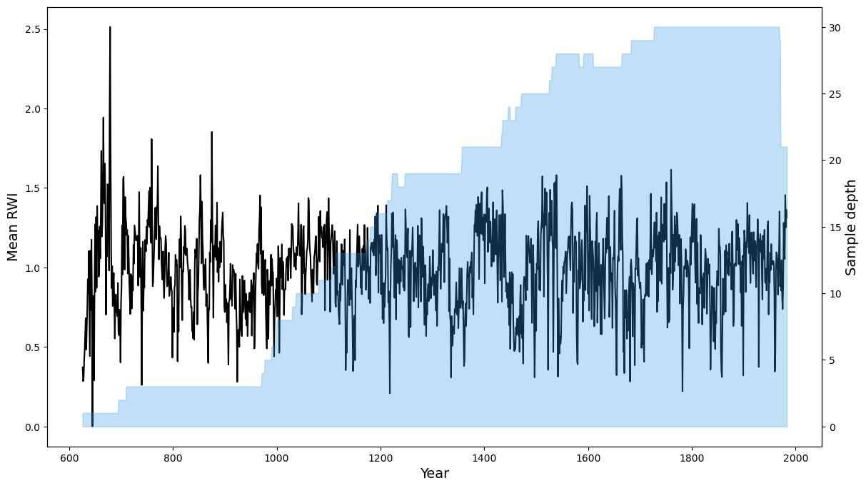
chron
Summary
Creates a mean value chronology for a dataset, typically the ring width indices of a detrended series. Takes three optional arguments biweight, prewhiten, and plot. They determine whether to find means using Tukey's bi-weight robust mean (default True), whether to prewhiten data by fitting to an AR model (default False), and whether to plot the results of the chronology (default True).
Parameters
-
data: a pandas dataframe - a pandas dataframe imported fromdpl.readers() -
biweight:boolean, defaultTrue- use Tukey's bi-weight robust mean -
prewhiten:boolean, defaultFalse- run pre-whitening on the time series -
plot:boolean, defaultTrue- plot the results
Examples
>>> dpl.chron(<data>, prewhiten=<True/False>, biweight=<True/False>, plot=<True/False>)
>>> import dplpy as dpl
>>> ca533 = dpl.readers("../tests/data/csv/ca533.csv")

# Detrending data first
>>> rwi_ca533 = dpl.detrend(ca533)

# Creating chronology using detrended data
>>> dpl.chron(rwi_ca533, prewhiten=False, biweight=True, plot=True)
Returns
The expected output is the mean value chronology of a specific dataframe.
The expected output from the example above will look similar to this:
        Mean RWI    Sample depth
Year
626     0.371605    1
627     0.284398    1
628     0.306523    1
629     0.416333    1
630     0.482462    1
...     ...         ...
1979    1.053427    21
1980    1.455353    21
1981    1.252526    21
1982    1.362244    21
1983    1.314827    21
1358 rows × 2 columns
If plot=True then a plot will also be generated:
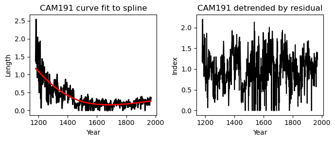
detrend
Summary
Detrends a given series or dataframe, first by fitting data to curve(s), with spline as the default, and then by calculating residuals (default = residual) or differences (difference) compared to the original data. Other supported curve fitting methods are ModNegex (modified negative exponential), Hugershoff, linear, horizontal.
Parameters
-
data: a pandas dataframe - a pandas dataframe imported fromdpl.readers() -
series:str- an individual series within a chronologydatafile. -
fit:str, defaultspline- fitting method of curves, e.g.,horizontal,Hugershoff,linear,ModNegex(modified negative exponential), andspline. -
method:str, defaultresidual- intercomparison method, options:differenceorresidual. -
plot:boolean, defaultTrue- plot the results.
Examples
>>> import dplpy as dpl
>>> data = dpl.readers("../tests/data/csv/file.csv")
>>> dpl.detrend(data)
# Detrending a series part of the dataframe
>>> dpl.detrend(data["<series>"])
# Detrending function and its options
>>> dpl.detrend(data["<series>"], fit="<fitting method>", method="<comparison method>", plot=<True/False>)
Returns
The expected output is the a list of detrended values (for the entire dataset or for a specific series)
The expected output from the example above will look similar to this:
1180    1.180835
1181    1.511543
1182    1.870558
1183    2.197630
1184    1.815025
        ...
1966    1.060515
1967    1.209514
1968    1.282459
1969    1.392746
1970    1.239629
Name: CAM191, Length: 791, dtype: float64
If plot=True then a plot will also be generated:
help
Summary
Python includes a built in help() functionality.
Use help() to read the documentation for each dplpy function.
Examples
>>> help(dpl.readers)
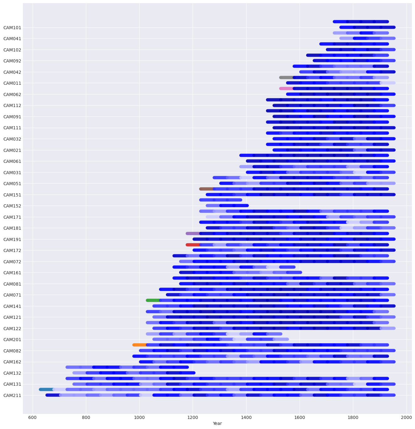
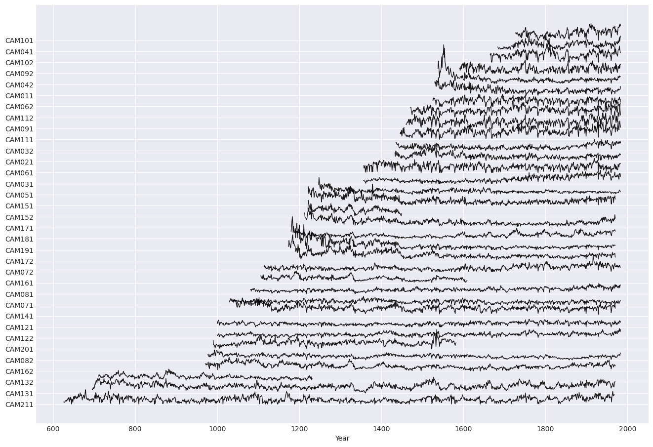
plot
Summary
Plots a given dataframe or series of a specific dataframe in either line (default), spaghetti (spag) or segment (seg) plots.
Parameters
-
data: a pandas dataframe - a pandas dataframe imported fromdpl.readers() -
series:str- an individual series within a chronologydatafile. -
type:str- type of plot to generate, e.g.,line, spaghetti (spag), or segment (seg). defaultline
Examples
>>> dpl.plot(<data>)
# Plot series subset of dataframe with a specified plot type
>>> dpl.plot(<data>["<series>"], type=<plot type>)
Returns
A graph of the specified dataframe.
From the example above, the expected output would look something similar to the below plot:
rbar
Summary
Finds best interval of overlapping series over a long period of years and calculates rbar constant for a dataset. Supports a number of rbar methods: osborn, 67spline, frank.
Parameters
-
data: a pandas dataframe - a pandas dataframe imported fromdpl.readers() -
start:int- start date year -
end:int- end date year -
method:strdefaultosborn- rbar method, optionsosborn,67spline,frank.
Further development underway. Future versions to prioritize number of series, number of years or both. Current version attempts to do both.
Examples
# Detrend data
>>> rwi_data = dpl.detrend(<data>, plot=False)

# Find common interval of detrended data
>>> start, end = dpl.common_interval(<data>)

# Calculate rbar coonstant
>>> dpl.rbar(rwi_data, start, end, method="<rbar method>")
Example:
# Detrend data
>>> rwi_data = dpl.detrend(ca533, plot=False)

# Find common interval of detrended data
>>> start, end = dpl.common_interval(ca533)

# Calculate rbar coonstant using the interval calculated above and using the Osborn method
>>> dpl.rbar(rwi_data, start, end, method="osborn")
Returns
rbar returns a list of constants to multiply with each mean value generated for a range of years from a mean value chronology.
From the example above, the output is the following:
[0.44170725878965766,
0.44170725878965766,
0.44170725878965766,
0.44170725878965766,
0.44170725878965766,
0.44170725878965766,
...
0.44170725878965766,
0.44170725878965766,
0.44170725878965766,
0.44170725878965766,
0.44170725878965766]
readers
Summary
This function imports common ring width data files (.CSV, .RWL) into Python as arrays
Parameters
data: a pandas dataframe - a pandas dataframe imported fromdpl.readers()
Supported data types
dplPy currently supports `csv` and `rwl` data formats.
Examples
>>> import dplpy as dpl
>>> data = dpl.readers("../tests/data/csv/file.csv")
>>> data = dpl.readers("../tests/data/csv/file.rwl", header=True)
Returns
- A success message;
- A list of series within the data file such as the following:
Attempting to read input file: ca533.rwl as .rwl format

SUCCESS!
File read as: .rwl file

Series names:
['CAM011', 'CAM021', 'CAM031', 'CAM032', 'CAM041', 'CAM042', 'CAM051', 'CAM061', 'CAM062', 'CAM071', 'CAM072', 'CAM081', 'CAM082', 'CAM091', 'CAM092', 'CAM101', 'CAM102', 'CAM111', 'CAM112', 'CAM121', 'CAM122', 'CAM131', 'CAM132', 'CAM141', 'CAM151', 'CAM152', 'CAM161', 'CAM162', 'CAM171', 'CAM172', 'CAM181', 'CAM191', 'CAM201', 'CAM211']
readme
Parameters
The readme function opens the opendendro webpage.
Examples
>>> dpl.readme()
Returns
This website opens!
report
Summary
Generates a report about the input dataset that includes:
- Number of dated series
- Number of measurements
- Avg series length (years)
- Range (total years)
- Span (start-end year)
- Mean (Standard Deviation) series intercorrelation
- Mean (Standard Deviation) AR1
- Years with absent rings listed by series
Parameters
data: a pandas dataframe - a pandas dataframe imported fromdpl.readers()
Examples
>>> import dplpy as dpl
>>> data = dpl.readers("../tests/data/csv/file.csv")
>>> dpl.report(data)
Returns
From the example above, the expected output is the following:
Number of dated series: 34
Number of measurements: 23276
Avg series length: 684.5882
Range: 1358
Span: 626 - 1983
Mean (Std dev) series intercorrelation:
Mean (Std dev) AR1: 0.7122
-------------
Years with absent rings listed by series

    CAM011 -- 1753 1782
    CAM031 -- 1497 1500 1523 1533 1540 1542 1545 1578 1579 1580 1655 1668 1670 1681
    CAM032 -- 1497 1523 1579 1654 1670 1681 1782
    CAM051 -- 1475
    CAM061 -- 1497 1523 1542 1545 1547 1579 1654 1655 1668 1670 1672 1782 1858 1960
    CAM062 -- 1542 1545 1547 1548 1579 1654 1655 1670 1672 1782 1836 1857 1858 1929
    CAM071 -- 1269 1497 1498 1523 1542 1547 1578 1579 1612 1655 1656 1668 1670 1672 1674 1690 1707 1708 1756 1782 1795 1820 1836 1845 1857 1858 1924 1948 1960
    CAM072 -- 1218 1497 1498 1523 1533 1538 1542 1545 1546 1547 1571 1579 1580 1590 1654 1655 1668 1670 1672 1675 1690
    CAM081 -- 1218 1336
    CAM082 -- 1362 1858 1865
    CAM091 -- 1655 1669 1670 1782 1858
    CAM092 -- 1624 1654 1655 1670 1672 1675 1677 1690 1703 1705 1707 1708 1710 1733 1753 1756 1757 1774 1777 1781 1782 1783 1784 1795 1807 1824 1829 1836 1845 1857 1858 1899 1904 1929 1936 1961
    CAM101 -- 1782 1783 1899 1929
    CAM102 -- 1669 1690 1782 1858 1899 1929
    CAM111 -- 1542
...
    CAM201 -- 1523
    CAM211 -- 645 762 809 847 924 957 1014 1118 1123 1133 1147 1189 1350 1384 1468 1571 1641
-------------
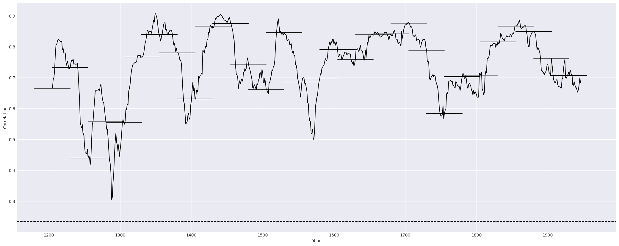
series_corr
Summary
Crossdating function that focuses on the comparison of one series to the master chronology.
Parameters
-
data: a pandas dataframe - a pandas dataframe imported fromdpl.readers() -
series:str- an individual series within a chronologydatafile. -
prewhiten:booleandefaultFalse- run pre-whitening on the time series, options:TrueorFalse. -
corr:str, defaultSpearman- select correlation type ifprewhiten=True, options:PearsonorSpearman. -
seg_length:intdefault50- segment length (years). -
bin_floor:intdefault100- select bin size. -
p_val:doubledefault0.05- select a p-value, e.g.,0.05,0.01,0.001. -
plot:booleandefaultTrue- plot the output.
Examples
>>> dpl.series_corr(ca533, "CAM191", prewhiten=False, corr="Pearson", bin_floor=10)
Returns
Two graphs: the first graph showing the correlation of one series to against the master chronology in a line graph; the second graph supports the first, showing the correlation in segments. For the example above, the graphs are as following:
stats
Summary
Generates summary statistics for rwl and csv format files. It outputs a table with first, last, year, mean, median, stdev, skew, gini, ar1 for each series in data file.
Parameters
data: a pandas dataframe - a pandas dataframe imported fromdpl.readers()
Examples
>>> dpl.stats(<data>)
>>> dpl.stats(ca533)
Returns
Table with first, last, year, mean, median, stdev, skew, gini, ar1 for each series in data file. For the example above, the output table is the following:
    series  first   last    year    mean    median  stdev   skew    gini    ar1
1   CAM011  1530    1983    454     0.440   0.40    0.222   1.029   0.273   0.698
2   CAM021  1433    1983    551     0.424   0.40    0.185   0.946   0.237   0.702
3   CAM031  1356    1983    628     0.349   0.29    0.214   0.690   0.341   0.809
4   CAM032  1435    1983    549     0.293   0.26    0.163   0.717   0.309   0.665
5   CAM041  1683    1983    301     0.526   0.53    0.223   0.488   0.238   0.710
6   CAM042  1538    1983    446     0.439   0.36    0.348   3.678   0.324   0.881
7   CAM051  1247    1983    737     0.273   0.25    0.140   1.836   0.262   0.705
8   CAM061  1357    1983    627     0.462   0.47    0.202   -0.111  0.247   0.510
9   CAM062  1525    1983    459     0.442   0.45    0.188   -0.266  0.240   0.529
10  CAM071  1037    1983    947     0.249   0.25    0.109   0.027   0.247   0.578
11  CAM072  1114    1983    870     0.309   0.29    0.163   0.698   0.292   0.735
12  CAM081  1081    1983    903     0.327   0.31    0.124   0.555   0.211   0.723
13  CAM082  977     1983    1007    0.285   0.29    0.114   0.312   0.223   0.771
14  CAM091  1460    1983    524     0.532   0.52    0.255   0.425   0.267   0.632
15  CAM092  1591    1983    393     0.349   0.34    0.226   0.337   0.369   0.561
16  CAM101  1727    1983    257     0.568   0.56    0.260   0.254   0.259   0.716
17  CAM102  1665    1983    319     0.604   0.62    0.261   0.082   0.243   0.677
18  CAM111  1446    1983    538     0.625   0.62    0.249   0.196   0.225   0.625
19  CAM112  1471    1983    513     0.570   0.56    0.211   0.223   0.207   0.583
20  CAM121  1000    1983    984     0.259   0.26    0.106   0.042   0.231   0.594
21  CAM122  1000    1983    984     0.271   0.27    0.109   0.346   0.223   0.653
22  CAM131  695     1970    1276    0.552   0.53    0.198   0.330   0.202   0.788
23  CAM132  710     1232    523     0.397   0.38    0.148   0.871   0.203   0.810
24  CAM141  1030    1970    941     0.627   0.60    0.204   0.695   0.177   0.746
25  CAM151  1222    1970    749     0.446   0.39    0.273   1.068   0.332   0.765
26  CAM152  1221    1449    229     0.534   0.52    0.195   0.297   0.203   0.695
27  CAM161  1106    1609    504     0.339   0.33    0.149   0.633   0.243   0.794
28  CAM162  971     1970    1000    0.397   0.37    0.184   0.647   0.259   0.840
29  CAM171  1213    1970    758     0.450   0.40    0.210   1.250   0.250   0.799
30  CAM172  1174    1970    797     0.482   0.42    0.249   1.622   0.268   0.847
31  CAM181  1190    1970    781     0.283   0.25    0.149   0.706   0.293   0.805
32  CAM191  1180    1970    791     0.366   0.25    0.336   2.359   0.429   0.876
33  CAM201  990     1582    593     0.474   0.47    0.181   0.772   0.208   0.709
34  CAM211  626     1968    1343    0.357   0.34    0.182   0.513   0.286   0.683
summary
Summary
The summary function generates a summary of each series recorded in rwl and csv format files. It outputs a table with count, mean, std, min, 25%, 50%, 75%, max for each series in data file.
Parameters
data: a pandas dataframe - a pandas dataframe imported fromdpl.readers()
Examples
>>> import dplpy as dpl
>>> data = dpl.readers("../tests/data/csv/file.csv")
>>> dpl.summary(data)
Returns
Summary outputs a table with count, mean, std, min, 25%, 50%, 75%, max for each series in data file. For the example above, the output table is the following:
        CAM011      CAM021      CAM031      CAM032      CAM041      CAM042      CAM051      CAM061      CAM062      CAM071      ... CAM151      CAM152      CAM161      CAM162      CAM171      CAM172      CAM181      CAM191      CAM201      CAM211
count   454.000000  551.000000  628.000000  549.000000  301.000000  446.000000  737.000000  627.000000  459.000000  947.000000  ... 749.000000  229.000000  504.000000  1000.000000 758.000000  797.000000  781.000000  791.000000  593.000000  1343.000000
mean    0.439581    0.424465    0.349156    0.293224    0.525648    0.439148    0.273012    0.462281    0.441939    0.249071    ... 0.445648    0.533799    0.339464    0.396710    0.450264    0.482296    0.282638    0.366271    0.473929    0.356813
std     0.221801    0.185397    0.213666    0.162930    0.222568    0.347705    0.139691    0.201785    0.188389    0.109357    ... 0.272561    0.194947    0.148916    0.184057    0.209848    0.249002    0.148853    0.335788    0.180967    0.182086
min     0.000000    0.050000    0.000000    0.000000    0.100000    0.070000    0.000000    0.000000    0.000000    0.000000    ... 0.000000    0.060000    0.000000    0.000000    0.080000    0.080000    0.000000    0.000000    0.000000    0.000000
25%     0.290000    0.290000    0.180000    0.180000    0.350000    0.270000    0.180000    0.335000    0.330000    0.180000    ... 0.240000    0.410000    0.230000    0.260000    0.300000    0.310000    0.170000    0.170000    0.350000    0.220000
50%     0.400000    0.400000    0.290000    0.260000    0.530000    0.360000    0.250000    0.470000    0.450000    0.250000    ... 0.390000    0.520000    0.330000    0.370000    0.400000    0.420000    0.250000    0.250000    0.470000    0.340000
75%     0.540000    0.520000    0.510000    0.390000    0.680000    0.460000    0.330000    0.600000    0.580000    0.320000    ... 0.610000    0.660000    0.430000    0.510000    0.580000    0.590000    0.380000    0.455000    0.580000    0.470000
max     1.360000    1.110000    1.030000    0.850000    1.380000    3.030000    1.320000    1.090000    0.920000    0.620000    ... 1.640000    1.250000    0.900000    1.040000    1.540000    1.980000    0.800000    2.540000    1.490000    1.100000
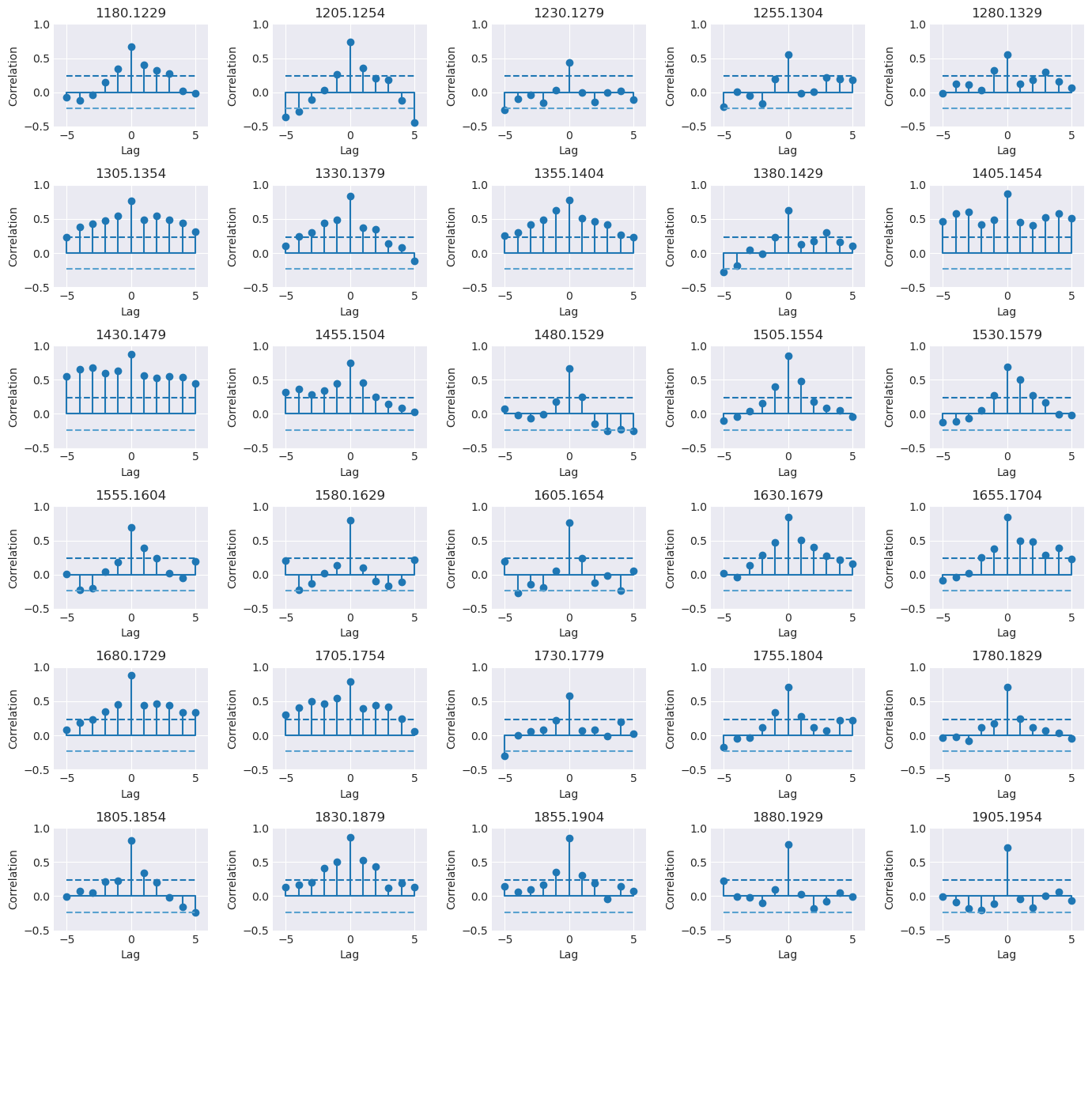
xdate
Summary
Crossdating function for dplPy datasets.
Parameters
-
data: a pandas dataframe - a pandas dataframe imported fromdpl.readers() -
prewhiten:booleandefaultTrue- prewhiten series using AR modeling -
corr:strdefaultSpearman- correlation type, options: 'Pearson' or 'Spearman' -
slide_period:intdefault50- period window (years) -
bin_floor:intdefault100- bin size -
p_val:floatdefault0.05- p-value, options: '0.05', '0.01', '0.001' -
show_flags:booleandefaultTrue- show flags in the output
Examples
>>> ca533_rwi = dpl.detrend(ca533, fit="spline", method="residual", plot=False)
# Crossdating of detrended data
>>> dpl.xdate(ca533_rwi, prewhiten=True, corr="Spearman", slide_period=50, bin_floor=100, p_val=0.05, show_flags=True)
Expected outputs
Outputs a dataframe of each series' segment correlations compared to the same segments in the master chronology.
For the above example, the expect output dataframe is the following:
Flags for CAM011
[B] Segment  High   -10    -9    -8    -7    -6    -5    -4    -3    -2    -1     0    +1    +2    +3    +4    +5    +6    +7    +8    +9   +10
1900-1949    6 -0.03 -0.31  0.17 -0.17  0.03 -0.18 -0.15  0.09 -0.16  0.20  0.15 -0.08 -0.03  0.08  0.13 -0.06  0.30  0.20 -0.17  0.09 -0.04

Flags for CAM051
[B] Segment  High   -10    -9    -8    -7    -6    -5    -4    -3    -2    -1     0    +1    +2    +3    +4    +5    +6    +7    +8    +9   +10
1375-1424    9 -0.02 -0.21  0.29  0.10 -0.09  0.06  0.30  0.09 -0.01 -0.03  0.18 -0.03 -0.16  0.24 -0.05 -0.06 -0.03  0.03 -0.11  0.38 -0.11

Flags for CAM131
[A] Segment  High   -10    -9    -8    -7    -6    -5    -4    -3    -2    -1     0    +1    +2    +3    +4    +5    +6    +7    +8    +9   +10
1800-1849    0 -0.13 -0.13 -0.05  0.05  0.09 -0.03 -0.14 -0.16 -0.00 -0.25  0.13 -0.11  0.10 -0.15  0.01 -0.34  0.09 -0.01  0.09 -0.09  0.05

Flags for CAM171
[B] Segment  High   -10    -9    -8    -7    -6    -5    -4    -3    -2    -1     0    +1    +2    +3    +4    +5    +6    +7    +8    +9   +10
1275-1324   -4 -0.04  0.00 -0.11  0.01 -0.05 -0.05  0.46  0.27 -0.13  0.02  0.28  0.23  0.01  0.20  0.12 -0.04  0.03 -0.14  0.01  0.01 -0.13

Flags for CAM181
[B] Segment  High   -10    -9    -8    -7    -6    -5    -4    -3    -2    -1     0    +1    +2    +3    +4    +5    +6    +7    +8    +9   +10
1775-1824    8 -0.13  0.05  0.07 -0.06 -0.12  0.19  0.14 -0.36 -0.30  0.06  0.21 -0.02 -0.15  0.16  0.14 -0.05 -0.02 -0.01  0.31  0.05 -0.14

Flags for CAM201
[A] Segment  High   -10    -9    -8    -7    -6    -5    -4    -3    -2    -1     0    +1    +2    +3    +4    +5    +6    +7    +8    +9   +10
1350-1399   -7 -0.04  0.03 -0.05  0.25 -0.08 -0.09 -0.13  0.01 -0.08  0.22  0.19  0.17 -0.13  0.13  0.09 -0.14 -0.26  0.03 -0.15 -0.14  0.12
[B] Segment  High   -10    -9    -8    -7    -6    -5    -4    -3    -2    -1     0    +1    +2    +3    +4    +5    +6    +7    +8    +9   +10
1125-1174    1 -0.02 -0.03 -0.12 -0.17 -0.08  0.08  0.18  0.00  0.19 -0.27  0.28  0.39  0.12 -0.24  0.01 -0.06 -0.15 -0.00 -0.10 -0.14 -0.18
...
1000-1049   -1  0.04  0.07 -0.16 -0.06  0.09 -0.07 -0.24 -0.12 -0.04  0.45  0.30 -0.33 -0.14  0.06  0.18 -0.06 -0.27 -0.25  0.09  0.12  0.16
1025-1074   -1  0.02 -0.19 -0.08 -0.08 -0.20 -0.09 -0.18 -0.18  0.19  0.70  0.36 -0.15 -0.01  0.08 -0.13 -0.34 -0.27 -0.14 -0.04  0.11  0.15

# Dataframe is truncated for visualization purposes
            CAM011      CAM021      CAM031      CAM032      CAM041      CAM042      CAM051      CAM061      CAM062      CAM071      ... CAM151      CAM152  CAM161  CAM162      CAM171      CAM172      CAM181      CAM191      CAM201  CAM211
700-749     NaN         NaN         NaN         NaN         NaN         NaN         NaN         NaN         NaN         NaN         ... NaN         NaN     NaN     NaN         NaN         NaN         NaN         NaN         NaN     0.402641
725-774     NaN         NaN         NaN         NaN         NaN         NaN         NaN         NaN         NaN         NaN         ... NaN         NaN     NaN     NaN         NaN         NaN         NaN         NaN         NaN     0.459880
750-799     NaN         NaN         NaN         NaN         NaN         NaN         NaN         NaN         NaN         NaN         ... NaN         NaN     NaN     NaN         NaN         NaN         NaN         NaN         NaN     0.303433
1775-1824   0.482449    0.526435    0.294118    0.646002    0.451140    0.489364    0.455558    0.777575    0.862473    0.772677    ... 0.702473    NaN     NaN     0.484946    0.572821    0.578103    0.208547    0.764706    NaN     0.544202
1800-1849   0.522305    0.456999    0.308715    0.568499    0.581273    0.485234    0.607107    0.790732    0.810612    0.761633    ... 0.782953    NaN     NaN     0.532389    0.523073    0.749052    0.256567    0.810900    NaN     0.568980
1825-1874   0.545834    0.575606    0.546987    0.625834    0.655030    0.514622    0.572533    0.793421    0.747419    0.652533    ... 0.707275    NaN     NaN     0.494070    0.535942    0.700264    0.411092    0.736471    NaN     0.503770
1850-1899   0.538631    0.738295    0.656855    0.714382    0.652629    0.655414    0.402929    0.859112    0.801489    0.674430    ... 0.692101    NaN     NaN     0.567827    0.538151    0.672989    0.513661    0.749436    NaN     0.660120
1875-1924   0.302665    0.751164    0.533637    0.640816    0.461801    0.604994    0.425498    0.709196    0.716879    0.653493    ... 0.689508    NaN     NaN     0.717551    0.542185    0.692869    0.554094    0.679136    NaN     0.683361
1900-1949   0.153806    0.700456    0.640816    0.696230    0.465738    0.728307    0.385162    0.647155    0.718703    0.493013    ... 0.730612    NaN     NaN     0.628523    0.575222    0.751068    0.423866    0.728307    NaN     0.566963
1925-1974   0.288836    0.618439    0.560912    0.688547    0.509724    0.637935    0.354238    0.696711    0.813205    0.529220    ... NaN         NaN     NaN     NaN         NaN         NaN         NaN         NaN         NaN     NaN
xdate_plot
Summary
Function is under construction
Visualize crossdating function in plot form; Each segment correlation is color coded.
Parameters
data: a pandas dataframe - a pandas dataframe imported fromdpl.readers()
Examples
dpl.xdate_plot(<data>)
# Detrend data first
ca533_rwi = dpl.detrend(ca533, fit="spline", method="residual", plot=False)

# Crossdating of detrended data
dpl.xdate_plot(ca533_rwi)
Returns
A graph showing segment correlations.